I. Contents

• Neural Dependency Parsing
  • Neural Dependency Parsing
  • A bit more about neural Networks
• Language Modeling and RNNs
  • Language Modeling
  • N-grams Language Models
  • Neural Language Models
  • Evaluating Language Models
• LSTM : Long Short-Term Memory RNNs
  • Problems with Vanishing and Exploding Gradients
  • LSTMs
  • More about vanishing/exploding gradient Problem
  • Bidirectional and Multi-layer RNNs: Motivation
• Summary

II. Neural Dependency Parsing

1. Neural Dependency Parsing

Deep learning classifiers are non-linear classifiers (cf. Traditional ML classifiers only give linear decision boundaries)

A Fast and Accurate Dependency Parser using Neural Networks Chen and Manning, 2014

2. A bit more about neural networks

• Regularization
• Dropout
• Vectorization
• Non-linearities
• Parameter initialization
• Optimizers
• Learning rates

III. Language modeling and RNNs

1. Language Modeling

Language Modeling is the task of predicting what word comes next.

More formally: given a sequence of words \(x^{(1)},x^{(2)},\cdots,x^{(t)}\), compute the probability distribution of the next word \(x^{(t+1)}\)

\[P(x^{(t+1)}\mid x^{(t)},\cdots x^{(1)})\]

where \(x^{(t+1)}\) can be any word in the vocabulary \(V = {w_1, \cdots , w_{\mid V\mid }}\)

주어진 단어들의 sequence가 있을 때, 그 다음에 올 단어의 확률분포를 구하는 것을 Language modeling이라고 한다.

각 sequence step마다 “단어가 다음에 올 확률”을 곱하면 전체 텍스트의 확률 분포가 되며, 식은 아래와 같다.

\[P(x^{(1)},\cdots ,x^{(T)})=P(x^{(1)})\times P(x^{(2)\mid x^(1)}) \times \cdots \ = \prod_{t=1}^T P(x^{(t)}\mid x^{(t-1)},\cdots ,x^{(1)}) \]

2. N-gram Language Models

Idea : Collect statistics about how frequent different n-grams are and use these to predict next word.

First we make a Markov assumption : \(x^{(t+1)}\) depends only on the preceding \(n-1\) words

\[P(x^{(t+1)}\mid x^{(t)},\cdots x^{(1)}) = P(x^{(t+1)}\mid x^{(t)},\cdots x^{(t-n+2)}) \ = \frac {P(x^{(t+1)},x^{(t)},\cdots x^{(t-n+2)})} {P(x^{(t)},\cdots x^{(t-n+2)})} \]

\[\approx \frac {count(x^{(t+1)},x^{(t)},\cdots x^{(t-n+2)})} {count(x^{(t)},\cdots x^{(t-n+2)})}\]

Problems of N-gram

• Sparsity Problems
  • Problem 1 : 위 식에서 분자 부분의 count가 0이라면, 해당 단어의 확률이 0으로 고정됨
    Solution : Add small \(\delta\) to the count for every \(w \in V\)
  • Problem 1 : 위 식에서 분모 부분의 count가 0이라면, 그 다음 단어의 확률을 정의할 수 없음
    Solution : 마지막 단어 하나 생략하고 찾기
• Storage Problems
  • Need to store count for all n-grams you saw in the corpus.

Results : Surprisingly grammatical!

…but incoherent. We need to consider more than three words at a time if we want to model language well. But increasing n worsens sparsity problem, and increase model size.

3. Neural Language Models

(1) A fixed-window neural Language Model

A Neural Probabilistic Language Model, Y.Bengio, et al. (2000/2003)

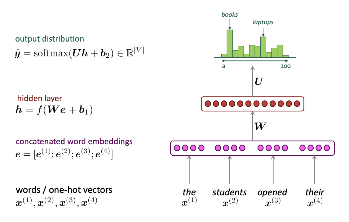
Improvements over n-gram LM

• No sparsity Problem
• Don’t need to store all observed n-grams

Remaining Problems

• Fixed window is too small
• Enlarging window enlarges \(W\) ☞ Window can never be large enough!
• No symmetry in how the inputs are processed

☞ We need a neural architecture that can process any length input!

(2) Recurrent Neural Networks

Core idea : Apply the same weights \(W\) repeatedly!

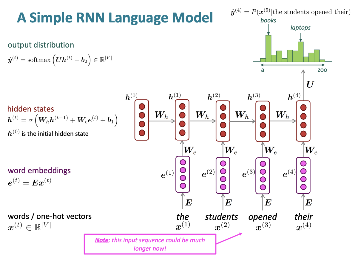
RNN Advantages

• Can process any length input
• Computation for step \(t\) can (in theory[due to gradient vanishing problem, “in theory”]) use information from many steps back
• Model size doesn’t increase for longer input context
• Same weights applied on every timestep, so there is symmetry in how inputs are processed.

RNN Disadvantages

• Recurrent computation is slow (it runs in the for loop, can’t be computed parallelly)
• In practice, difficult to access information from many steps back

Training an RNN Language Models

\[J^{(t)}(\theta)=CE(y^{(t)}, \hat y^{(t)})=-\sum_{w\in V}y_w^{(t)}=-log\hat y^{(t)}{x{t+1}}\]

\[J(\theta)=\frac {1}{T} \sum^T_{t=1}J^{(t)}(\theta)\]

4. Evaluating Language Models

The standard evaluation metric for LM is perplexity

\[perplexity = \prod_{t=1}^T (\frac {1}{P_{LM}(x^{(t+1)}\mid x^{(t)},\cdots ,x^{(1)})})^{1/T} \ = exp(J(\theta))\]

Lower perplexity is better!

probability of corpus의 기하평균의 역, 모든 단어를 정확히 맞춘다면 \(perplexity = 1\)

Why should we care about Language Modeling?

• Language Modeling is a benchmark task that helps us measure our progress on understanding language
• Language Modeling is a subcomponent of many NLP tasks

IV. LSTM : Long Short-Term Memory RNNs

1. Problems with Vanishing and Exploding Gradients

Vanishing gradients

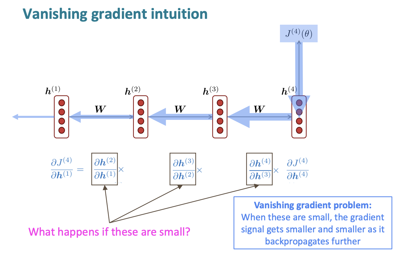
Exploding gradients

Exploding gradients can solve by simple methods such as gradient clipping .

How about a RNN with separate memory to fix the vanishing gradient problem? ☞ LSTMs

2. LSTMs

Hochreiter and Schmidhuber(1997)

Gers et al(2000) -> Crucial part of the modern LSTM is here!

On step \(t\), there is a hidden state \(h^{(t)}\) and a cell state \(c^{(t)}\)

• Both are vectors length \(n\)
• The cell stores long-term information
• The LSTM can read, erase, and write information from the cell
  • the cell becomes conceptually rather like RAM in a computer

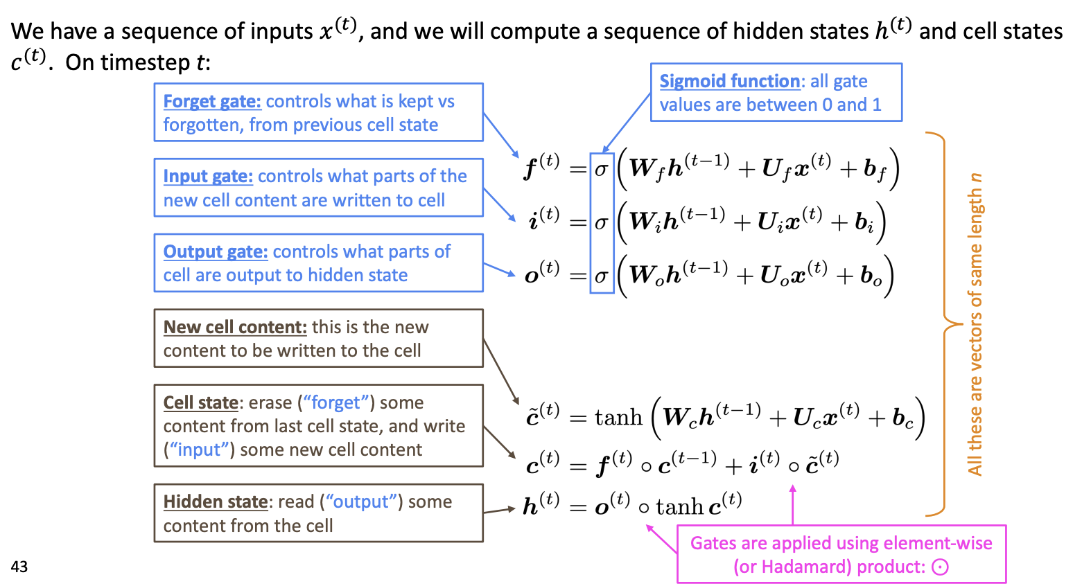
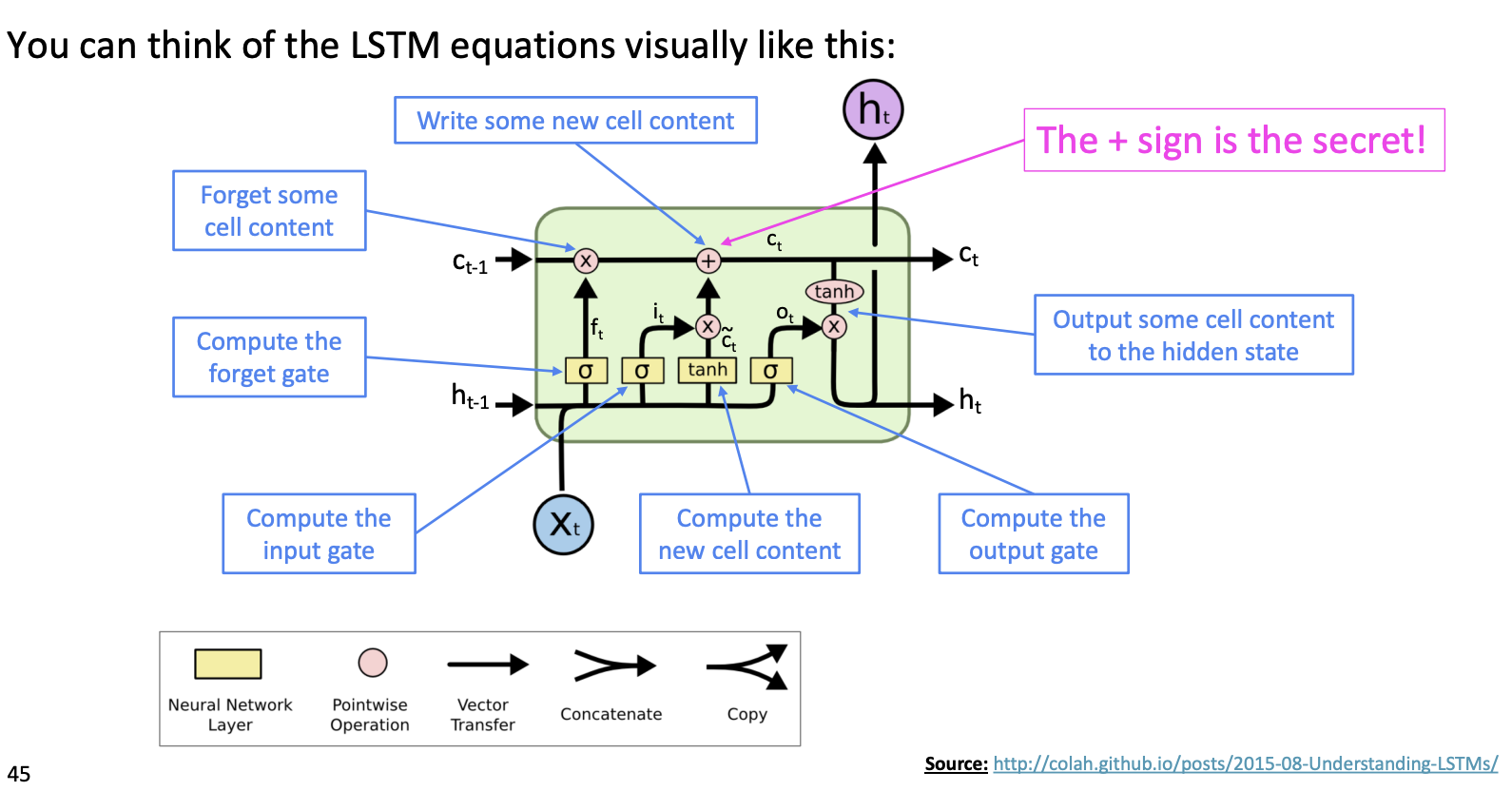
LSTM이 Gradient vanishing을 해결할 수 있는 핵심 구조는 cell state이다. cell state는 곱연산이 아닌 합연산을 통해 다음 cell로 전해지므로, step을 오래 거치더라도 vanishing이 발생하지 않는다.

cell state에 long term memory가 저장되므로, hidden state를 계산할 때 output gate를 통해 long term memory에 저장된 정보를 얼마나 사용할지 결정할 수 있다.

3. More about vanishing/exploding gradient Problem

Is vanishing/exploding gradient just a RNN problem?

No! It can be a problem for all neural architectures, especially very deep ones

Solution : Add more direct connections (e.g. ResNet, DenseNet, HighwayNet, and etc.)

4. Bidirectional and Multi-layer RNNs: Motivation

(1) Bidirectional RNNs

문장 구조상, 뒤에 있는 단어들 까지 보아야 단어의 의미를 파악할 수 있는 경우가 있다. (e.g. the movie was “teriibly” exciting!, terribly가 긍정적인 의미로 사용되었음을 알기 위해서는 뒤의 exciting도 보아야 한다.)

\(h^{(t)}\) has the dimension of \(2d\) (\(d\) is the hidden size of FW or BW)

Note: Bidirectional RNNs are only applicable if you have access to the entire input sequence ☞ Not applicable to LM!

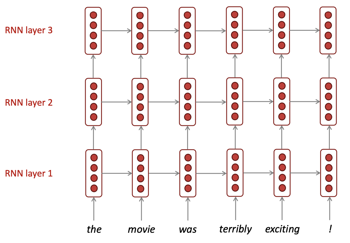
(2) Multi-layer RNNs

V. Summary

Language Modeling은 자연어처리에서 benchmark test & subcomponent 역할을 하는 task이다. 딥러닝 이전에 N-grams LM이 존재하였으며, RNN을 도입하면서 성능이 비약적으로 상승하였다.

한편, RNN의 특성상 gradient vanishing(exploding) 문제가 발생하는데, 이를 해결하기 위해 RNNs중 하나로서 LSTMs이 도입되었다. LSTM의 핵심은 long term memory를 저장하는 cell state로, 합연산을 통해 값이 전달되므로 vanishing이 현저하게 줄어든다.

RNNs의 성능을 더욱 향상시키기 위한 시도로 Bidirectional, Multi-layer RNNs 등이 있으며, 오늘날 가장 좋은 성능을 보이는 모델 중 하나인 BERT와 같은 Transformer-based network에서도 이러한 구조들을 채택하고 있다.